Neural Networks – Crash course
Today’s world cannot be envisioned anymore without the appliance of neural networks in our day-to-day life. Think about hand writing recognition, image recognition, voice recognition, recommendation engines etc. When we use our smartphones, our image gallery is automatically categorized and friends and family are automatically detected and tagged. To accomplish this our phone actually uses a neural network.
The rise of Neural Networks
Machine vision becomes more and more important, definitely in traffic for autonomous driving cars. It not only needs to classify images correctly and detect objects, people and situations but it also needs to do this extremely fast.
Luckily with todays hardware, this task becomes more and more trivial: the matrix calculations that are required to train and run neural networks can be put on graphical processors (GPUs). They are able to parallelize the workload and hence run complex neural networks. Today most smartphones dispose of GPU power and we can extend devices with GPU or TPU (Tensorflow Processing Unit) power.
While the hardware has taken flight, the same happened to the open-source community and its support and investment in Neural Network libraries, amongst which are Tensorflow, Keras, Pytorch and MXNet.
However, to understand this technology we first need to understand what a Neural Network is and what types of Neural Networks exist. And how they can be applied. So in this blog we’ll try to give a clear introduction in Neural Networks and how they work. This blog is of course not a complete and exhaustive overview of neural networks. The main purpose is to give you a clear overview of what a Neural Network actually does.
Structure of a Neural Network
Let’s have a look at a basic neural network architecture.
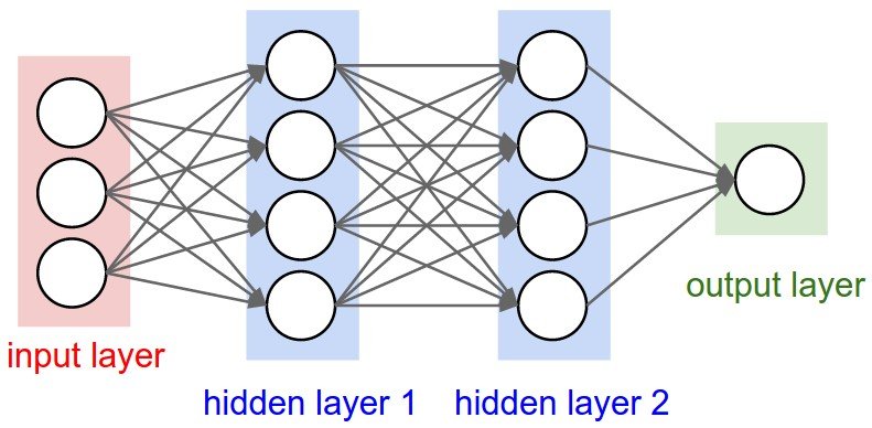
A neural network can be considered as a large calculation. It consists of an input layer, zero or more hidden (or processing) layers and an output layer.
At each node (or neuron) in the processing and output layer the following applies:
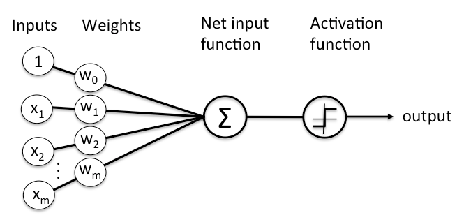
A node combines input from the data with a set of coefficients, also known as weights. These weights either amplify or dampen that input. As such they assign significance to inputs with regard to the task the algorithm is trying to learn.
These input-weight products are summed (and potentially a bias is added) and then the result is passed through a Neuron’s so-called activation function. The activation function will determine whether and to what extent that signal should progress further through the network to affect the ultimate outcome.
We actually have an input function like this: where
= the weight,
= the input and
is the bias.
An example Neural Network
Suppose we want our neural network to recognize some written numeric character (from 0 to 9). The input for the neural network is a frame of let’s say 28×28 pixels.
Each pixel has a gray value. Our neural network needs to calculate what’s on the picture and will do so by assigning all inputs, hence 28×28 = 784 gray values a value between 0 and 1. Notice that a neural network is not binary: each value in the neural network is a number between 0 and 1.
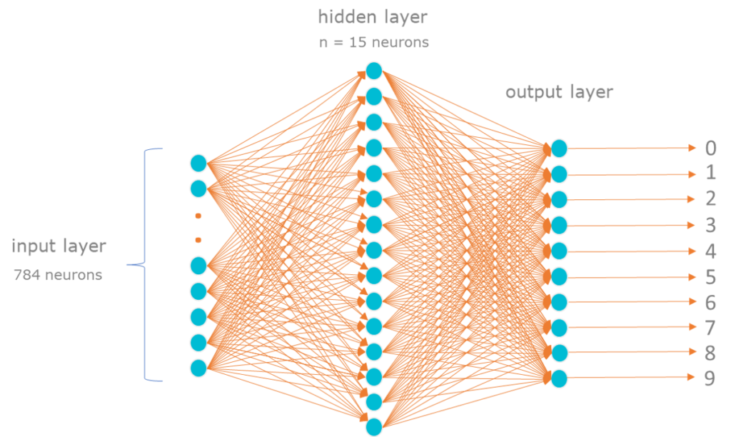
These data will be sent to the next ‘layer’, the hidden layer or processing layer. This layer consists of less neurons, let’s say 15. Each neuron in this layer gets input from the previous layer and assigns a weight to each input from the previous layer. The resulting value of this layer (again a value between 0 and 1) will be sent to the output layer and again assigned a weight. The neuron on this output layer that is closest to 1 will be marked as ‘detected’.
Assigning weights – Backpropagation
You might wonder how we assign these weights. A neural network, as described here above, with merely one processing layer, will have 784×15 (input -> hidden) + 15×10 (hidden -> output) weights. In addition each neuron can be assigned an additional weight (the bias at each neuron), hence 15 (hidden) + 10 (output) additional weights resulting in a total of 11935 weights or variables that we’ll need to manage and finetune. This looks like a daunting task and it’s definitely not feasible to do this manually.
The way we can ‘train’ these weights depends on the method chosen. In the above simple example of a feed-forward neural network we can train the network through supervised learning. We can feed the network with predefined frames of which we know the outcome. Any time the neural network produces an output we can compare it with the expected outcome and adjust the weights. The more the output deviates from the expected outcome, the more we need to adjust the weights. Each variable can receive a positive or negative vector to adjust the variable towards the expected outcome.
This process is called backpropagation. Mathematically speaking, gradients will be calculated to adjust the weights.
A gradient is the rate of change of a function. It’s a vector that points in the direction of greatest increase of a function. It’s the same as the derivative of a multi-variable function. We’ll dig a bit deeper further on this when discussing Optimizers.
Activation
To decide on each neuron whether its input will be forward fed, we need an activation function. Multiple activations exist like Sigmoid, ReLU etc. Activation functions will decide whether output will fire to the next neuron or not. Depending on the problem at hand a specific activation function is applicable. Look for example at the underlying activation functions:
 |
 |
| Sigmoid: |
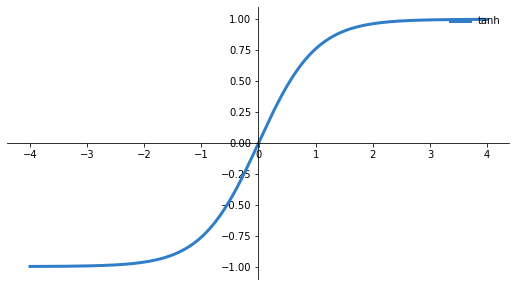
Tanh: |
 |
 |
| ReLU: |
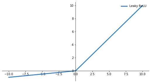
Leaky ReLU: |
The Sigmoid function looks good for classification purposes since it tends to bring the y values to either 1 or 0 (x > 2 or x < -2).
However there’s also an issue with this activation function. If you notice, towards either end of the sigmoid function, the Y values tend to respond very less to changes in X. This means that the gradient at that region is going to be small. This leads to the problem of “vanishing gradients”. If the gradient is small or has vanished, the network will not learn anymore or will become drastically slow.
Tanh is zero-centered compared to Sigmoid but also tends to saturate. ReLU doesn’t tend to saturate that much but still gradients can go to zero. Currently the most used activation functions are ReLU or variations of ReLU but Sigmoid is still very valuable in a lot of cases.
Everything depends on the problem at hand and which problem needs to be solved. The most important is to understand the characteristics of the activation function and to understand their impact on calculated gradients/weights on each layer of the NN.
Loss
To evaluate how well the network performs we need to calculate the loss (how far are we off with respect to the ground truth). Or in other words: how close is our predicted label to the actual label. This can be measured in multiple ways.
For instance MSE (Mean Squared Error) is a calculation used to calculate loss amongst all data points resulting in a single loss value:
MSE =
= observations,
= predictions
The purpose is then to minimize this cost function in order to be as close as possible to the actual values and hence finding the optimized values for weights.
Optimization
To do this we need to apply an Optimizer. Optimizers update the weight parameters to minimize the loss function. Again, multiple optimizers exist amongst which SGD (Stochastic Gradient Descent), NAG (Nesterov Accelerated Gradient), Adagrad (Adaptive Gradient Algorithm), Adam (Adaptive Moment Estimation) etc.
Gradient indicates the direction of increase. As we want to find the minimum point in the curve we need to go in the opposite direction of the gradient. Using derivatives, we can find the rate of change, or the slope, of a function at any point.
We update parameters in the negative gradient direction to minimize the loss. How this works can be seen in the animated picture below:
Of course it’s possible that a simple Gradient Descent optimizer will not find the global minimum but local minima (if the plane is much more complex than shown above). Hence why multiple Optimizers exist, with their pro’s and cons. It’s up to the data scientist to select the appropriate optimizer.
Hyperparameters
A hyperparameter is a variable who’s value is used to control the learning process of a machine learning model. In the case of a NN these are the parameters the NN can’t learn itself.
Training a NN will take multiple epochs. You can not train a network in 1 run. It will take multiple runs going forward and back before our loss will actually be optimized.
Training a NN will also involve batches of data. How much of your training data you use before you update the weights is defined by its batch size. It’s all an iterative process.
The number of epochs and the batch size are hyperparameters. Also the parameters that are required to tune the algorithm to optimize the cost function are hyperparameters, as are the number of layers and the number of neurons in each layer.
Underfitting and overfitting
If you feed the NN not enough representative data, the outcome will always be underfitting. Underfitting occurs when a statistical model or machine learning algorithm cannot capture the underlying trend of the data because it didn’t get enough data to learn from.
If you keep training it to be perfect to what you expect, it will overfit and will not be able to make a correct generalization. Overfitting occurs when a statistical model or machine learning algorithm captures the noise of the data.
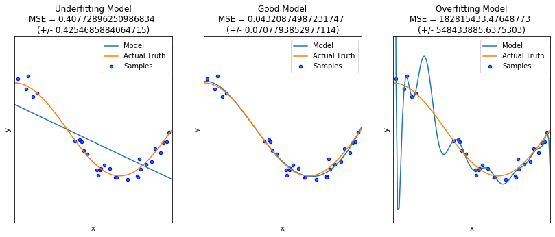
As you can see in the models above, the first model clearly underfits. The last model however clearly overfits: it will also include outliers/noise. You can see that we applied a cross-validation of the model through calculation of the MSE.
In the end, the purpose of a NN is to feed it data it didn’t see before and make a correct prediction based on what it has learnt. So we definitely don’t want an overfitting model.
Ok, so that was a brief summary of what Neural Networks are or at least what the most fundamental characteristics are of NNs. Let’s summarize:
Summary
In a neural network weights are calculated during training to provide a predicted output as close as possible to actual output.
An activation function will define whether or not an input will be forward fed.
Through backpropagation weights are adjusted.
The loss function will provide us a measure to verify how well the network performs, how close the predicted output is compared to the actual output.
To optimize the loss function we use an optimizer.
Key take aways:
Designing a neural network involves defining the number of layers and number of neurons in each layer, the activation functions for each layer, the loss function to measure its performance and the optimizer, and hyperparameters to optimize the loss and adjust the weights.
A NN requires training data. Datasets need to be split in training, test and validation sets. The data scientists must take care that the model will not underfit nor overfit.
The data scientist will also tune the hyperparameters of the NN.
Want to know more?
Get in Touch
Originally I started my career as an expert in OO design and development.
I shifted more than 15 years ago to data warehousing and business intelligence and specialised in big data and data science.
My main interests are in deep learning and big data technologies.
My mission: store, process and deliver data fast, provide insights in data, design ML models and apply them to smart devices.
In my spare time I’m very passionate about Salsa dancing. So much that I performed internationally and that I have my own dance school where I teach LA style salsa.